Let’s say you have a matrix $A$ of dimension (model_dim, n_samples), i.e. the columns correspond to points in a dataset. If we want to calculate PCA, we first center by subtracting the mean of the columns of $A$.

The classic PCA approach is to then get the covariance matrix $AA^T$ and take its eigendecomposition. From other notes we know that since the covariance matrix is symmetric, the eigendecomposition is equivalent to the SVD. So we have $U_{AA^T}\Sigma U_{AA^T}^T$ where my ugly subscripts are to be very clear that these are the singular vectors/eigenvectors of the covariance matrix; we can use the same matrix on both sides because it’s symmetric and it’s also an eigendecomposition.

We don’t actually have to calculate $AA^T$. We can directly take the SVD of $A$ instead as $U_A\Sigma V_A^T$. Then, we know that $AA^T=(U_A\Sigma V_A^T)(V_A\Sigma U_A^T)=U_A\Sigma^2U_A^T$ and that the left singular vectors of the data matrix $A$ are the same as the eigenvectors of $A$’s covariance matrix.

If you ever get confused about rows and columns, remember that you’d always want to take the singular vectors that are the model dimension; in this case they are the left singular vectors, since $A$ is (model_dim, n_samples). Also, the covariance matrix has to be (model_dim, model_dim).

Two ways to “project onto subspace”

If the columns of $A\in\mathbb{R}^{(d,n)}$ are all orthogonal vectors, then $AA^T$ is also the matrix that projects activations onto the $n$-dimensional subspace spanned by columns of $A$. (If they were not orthogonal vectors, the projection matrix would be $A(A^TA)^{-1}A^T$.) I can’t believe I never noticed this until now, need to think about deeper connections here.

There’s two ways to “project onto a subspace.” There’s the linear algebra 101 thing, where a matrix multiplication is a change of basis: so if I have a vector $v\in\mathbb{R}^d$ and multiply $A^Tv$, then that takes dot product of $v$ with each column of $A$, telling me “how much” that vector is in the direction of each of those columns (e.g. [0.2, 3.1]). We can reconstruct $v$ by just multiplying those coefficients by the columns of $A$ again: $A(A^Tv)$. But wait, we’ve actually lost information now about anything that can’t be spanned by the columns of $A$. That’s why $AA^T$ works as a projection matrix, if you want to only get the information in $v$ that’s in the subspace spanned by $A$’s columns, but keep that information in $d$ dimensions.

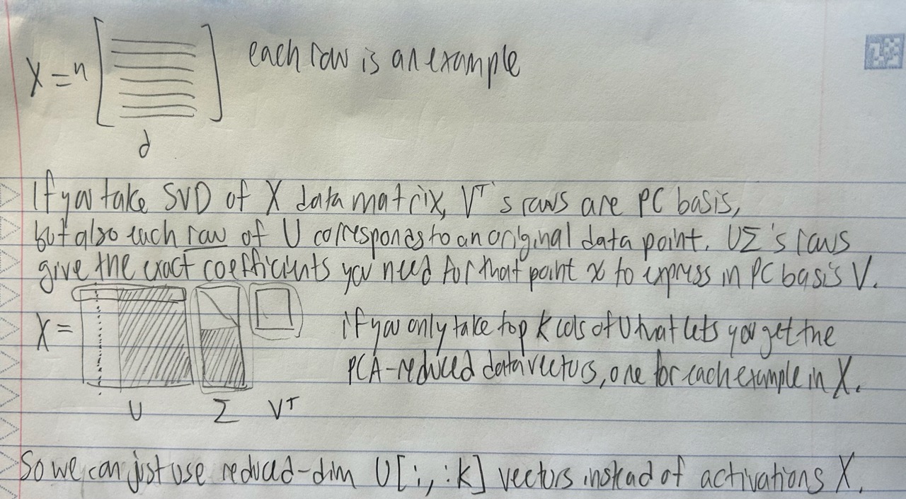
Interpreting the SVD of a Data Matrix X

This is restating half of the stuff above, but looking at the other set of singular vectors. Say you have a data matrix $X\in\mathbb{R}^{n\times d}$, where each of the $n$ rows is a data point (e.g. a hidden state) of $d$ dimensions (e.g., model dimension). Assuming that $X$ is centered, then if you take the SVD $X=U\Sigma V^T$, its $d$-dimensional singular vectors $V^T$ are also the principal components of the data, as we talked about above.

But then, how to interpret the $n$-dimensional singular vectors $U$? Well, since the rows of $X$ are all data points, each row of $U\Sigma$ corresponds to a data point in $X$. Specifically, each of those rows gives you that data point expressed in the principal component basis given by $V^T$ (i.e., the coefficients on $V^T$’s rows you need to construct that data point). So if you want to take the PCA-reduced version of the data in $X$, all you have to do is take the top-$k$ columns of $U\Sigma$, which automatically gives you a $n\times k$ matrix of $k$-dimensional vectors for every data point. This is super useful in practice; it’s an extremely quick way to project data onto the first $k$ principal dimensions.