Not All LM Features are 1D Linear (Engels et al., 2024)

[Paper, Video] - They’re basically trying to figure out how to decompose hidden states into sums of different functions of the input (features). So for example, you might have a 1-dimensional representation of an integer value 3, added to an n-dimensional representation of the language semantics of “three,” etc.

When you’re doing this, there’s a problem: how do you know whether a multi-dimensional feature you’ve found is “atomic”, or whether it’s actually possible to further decompose it into other sub-features?

Reducibility

To figure this out, they formally define reducible features—which crucially we don’t actually want to count as a good/valid multi-dimensional feature. So for a given multi-dimensional feature $\bf f$ (defined as a function that maps from inputs to some $d_f$-dimensional subspace), can it actually be “broken down” (e.g. latitude and longitude)?

They come up with two metrics to see if this is approximately true:

1. $S(f)$ - Separability index. For all possible ways to break down a feature into $\bf a$ and $\bf b$, what is the minimum mutual information $I(\textbf{a}, \textbf{b})$? For example, a multidimensional Gaussian will not actually have mutual information between subfeatures if you choose the right axes. Higher = harder to separate.
2. $M_\epsilon(f)$ - $\epsilon$-mixture index. Across all the token positions, can we pick a special vector $\bf v$ for which the feature can be projected near zero pretty often? (in practice, this is something like less than $\epsilon$ * standard deviation rather than zero). If you can find a vector $\bf v$ and offset $c$ so that $\textbf{v} \cdot \textbf{f(t)} + c$ is small for lots of token positions, then that means that in all of those cases that direction in the feature space wasn’t really being used. Of course, $\bf v$ has to be within the subspace $\mathbb{R}^{d_f}$, because otherwise you could easily find a vector that’s orthogonal to $\mathbb{R}^{d_f}$ and zeros out everything. Higher = easier to separate.

In practice, $S(f)$ scores for GPT-2 features are mostly less than 0.2 (aka, most features are pretty separable), and $M_\epsilon(f)$ features are quite high, mostly bigger than 0.4 (aka, most features are pretty much mixtures). They use these scores to argue that their day-of-week features, since they have high $S(f)$ and low $M_\epsilon(f)$, are irreducible multi-dimensional features.

Going from SAE to Multi-Dim Features

If $\bf D$ is the decoder matrix of the SAE containing all of the output features, then to cluster features together, they take the cosine similarity between all decoder vectors and prune away cosine similarities below a threshold $T$. By construction these clusters will be “$T$-orthogonal” (i.e. if $T=0$ then they’re truly orthogonal).

If the SAE is good at reconstructing, then when a multi-dimensional non-reducible feature $\bf f$ is active, they claim that one of these cosine-similar clusters will be equal to f. This is not super obvious. Naively, you’d think it’d be the opposite—that if $\bf f$ was a 2D feature that was properly reconstructed by the SAE, the SAE would have learned two orthogonal decoder vectors that span the space (and those would have close to zero cosine similarity). But if $\bf f$ is truly a multi-dimensional feature, it would never make sense to separate out these two features; then the SAE would get penalized by always having both features active whenever it needs to reconstruct $\bf f$. So instead, they guess that the SAE would learn a bunch of cosine-similar things that are all in $\bf f$ (intuitively, maybe this would be like learning separate “Monday”, “Tuesday”, “Wednesday” features).

So what they do is:

1. Cluster all the SAE decoder vectors using this thresholding thing
2. To analyze a cluster, get cluster-specific reconstructions of all hidden states $\textbf{x}_{i,l}$.
3. Analyze that cluster’s representations across a bunch of hidden states by looking at PCA projections, or running $S(f)$ and $M_\epsilon(f)$

Two important details:

• In order to calculate these scores, they actually first calculate the PCA directions over the reconstructed activations, and then project onto PCA components 1-2, 2-3, 3-4, 4-5, averaging the separability/mixture over each of these planes.
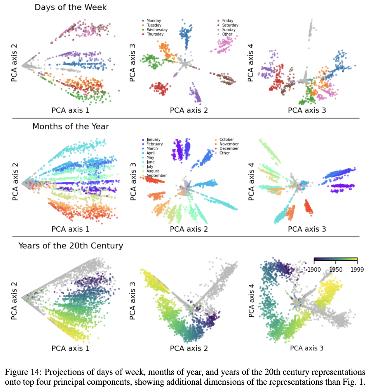
• This process implicitly filters for datapoints that are relevant for this cluster/feature. In step (2), if none of the cluster’s features are active for a particular hidden state $\textbf{x}_{i,l}$, it is not included in the analysis. In the case of a days-of-the-week feature, the PCAs will of course look pretty nice, since the biggest variation between a bunch of weekday vectors will almost surely be information about weekday.

Another cool thing is that they show that these features are actually cones, where the first principal component seems to be intensity of weekday-ness, perhaps.

Intervening on Circles

While they do try intervening on the subspace found by the SAE, they get slightly better results by training probes to find good subspaces at each layer. Specifically, they

1. Take the top-$k$ principal component directions of hidden states at the “Monday” position (pretty sure this position) across all the prompts and project onto there first.
2. Then train a linear probe $\bf P$ in that space that maps from $k$ to 2 dimensions, trained to correspond to circle($\alpha$) – e.g. for weekdays circle$(\alpha)=[\cos(2\pi\alpha/7), \sin(2\pi\alpha/7)]$.
3. To intervene on “Monday” and make it look like “Wednesday”, they just discard “Monday.” I am confused about how exactly this intervention works, because their Equation 6 seems wrong (you can’t calculate circle$(\alpha_{j’}) - \overline{x_{i,l}}$ directly because they are different dimensions). Equation 7 doesn’t clarify, it seems to have a missing parenthesis.

Josh Engels mentions in the talk that the intervention only works if you ablate out everything else that’s not in the PCA; I’m not exactly sure what he means here, probably the fact that they have to mean-ablate everything by using $\overline{x_{i,l}}$ instead of the base activation.

Generic Ideas/Takeaways

• How does the model actually use these circular representations to calculate the answer?
• Some of these facts must be piecewise memorized as well (e.g. Saturday is 1 day after Friday is almost surely memorized) – probably why they have to ablate all other weekday information.
• Presumably lots of weekday embedding information is unrelated to circles – if you rotated within the circle subspace for tasks like “What holidays are typically on [Thursday]?” or “What letter does [Thursday] start with?” then you’d probably see it doesn’t affect anything.
• It still worries me to think about multiple circles happening at once. If you have six orthogonal 2D circles, could that just be some alternate formulation of an n-dimensional subspace?

When Models Manipulate Manifolds / Linebreaks (Gurnee et al., 2025)

Line snaking through a subspace

They find 1-dimensional feature manifolds embedded in low-dimensional subspaces for: num. characters in a token, num. characters in current line, overall line width constraint, num characters remaining in the current line.

• It wouldn’t really make sense to dedicate an entire 1D subspace to num characters in current line, because then you’re wasting that entire dimension if you’re in a doc that doesn’t have linebreaks. This is really strong evidence for superposition; as they note, a ring structure implies that there is superposition/interference in that representation.

They find a bunch of features that activate on a range of given line widths. Since two are usually active at a time, they imagine a curve connecting all these features. If they take PCA across 150 different line width averages for Layer 2, they find a 6-dimensional subspace that explains 95% of the variance across line width averages. They can also reconstruct the activations only using the SAE features above, and the curves track each other fairly closely.

• This is really interesting because there is no human-intuitive reason why line widths would have to be represented as a curve, right? Unless there was something about a 60-length line that nicely parallels a 30-length line? This really might be an artifact of superposition, because we don’t want to use up an entire dimension, so we snake it around like so; probably because you’re unlikely to confuse 60 and 30 anyway(?)
• Q: do all of their averaged-line-width features come from tokens within documents with a max line width of 150, or do they come from different documents with different max line widths?
• If we were trying to find this using some geometric DAS, why would we assume we’re looking for a curved manifold? Or, how would we figure out what kind of curves we might be looking for? This seems like something someone who’s good at math could figure out

“Ringing” plots

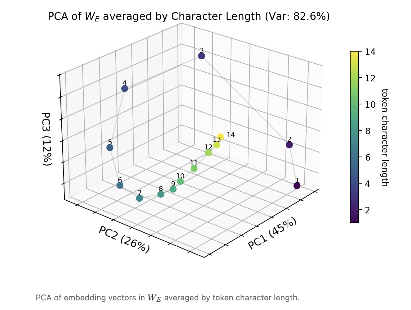
150-way logistic regression: basically just a bunch of model_dim vectors each individually trained to activate for e.g. a 50 char line, 51 char, etc. If they take all these guys and do PCA, the top 6 components capture 82% of the variance of these vectors. You can just plot the behavior of each of these logistic regression probes on a heatmap, and see that the diagonal is quite fuzzy. But you also see that there is some small off-diagonal “ringing” in their predictions as well (which also occurs if you take cosine sim. between all the mean vectors, or the probe vectors).

• A very fuzzy intuition for this is that if you have some representation of line width that snakes around within a subspace back onto itself, as well as a logistic regression probe vector that’s trained to have a high dot product with lines of a particular length, then it wouldn’t just slightly activate for adjacent line widths but also for areas near it on the spiral. (This is basically the intuition in their toy example.)

Math details for their toy model: let’s say we want 150 vectors that are all somewhat similar to their neighbors but orthogonal to everything else. They define the cosine similarity matrix $X$ for this toy setting as a “circulant matrix” where basically you just have the row [1, 0.5, 0, …] permuted to the right in every row to create a fuzzy diagonal. If you take a 5-rank approximation of it using the eigendecomposition of $X$, then you get the same “ringing” pattern. Note: it is nice to just look at the cosine similarity matrix here instead of trying to think of a familiar shape in 150 or 5 dimensions.

Probably the reason why they define $X$ to be circulant is because of its connection to Fourier transforms. Multiplying by a circulant matrix implements a convolution, which is just multiplication in Fourier space; this means that circulant matrices have eigenvectors that are Fourier modes (i.e., fundamental waves). So this approximation they were doing is equivalent to truncating the less-important Fourier coefficients for $X$.

Since this toy Fourier approximation looks so much like their real-life ringing example, they wonder whether the line width stuff in the real LLM is constructed via Fourier features. They say you can’t have just any generic low-dimensional embedding of a high-dimensional circle that slides along itself via a linear transform, which I buy. In the footnote they have this derivation about how this particular circulant matrix is built out of Fourier features, and show that because of this fact they are able to get a transformation on this structure that “slides it along itself.” For the actual character count curve, they find that Fourier approximations are pretty good at explaining the variance compared to ceiling (PCA).

Manipulation of Manifolds