They focus on a mod 113 model, finding key frequencies $k\in\{14,35,41,42,52\}$. How do they find these key frequencies?

Representing the Output Sum with Fourier Features

They do a lot of analysis on the “neuron-logit map,” $W_L\in\mathbb{R}^{|V|\times n}$, which is just the final MLP’s $W_{down}$ multiplied with $W_{unembed}$. Here, $|V|=113$ is the vocab size, and $n$ is the number of MLP neurons. They apparently find that the residual stream doesn’t matter in their toy model, it’s just MLP acts straight to the output logits. This is I think the most relevant place where they find the key frequencies.

• They do this by taking the discrete Fourier transform “across the logit axis,” i.e. from $\mathbb{R}^{|V|\times n}\rightarrow\mathbb{C}^{p\times n}$, where $p$ is the maximum period. This basically means they’re looking at how the signal oscillates as the number increases. Actually, $p=|V|$ because you can’t differentiate any periods that are greater than the number of numbers we have, but I’ll name them differently because they’re conceptually different.
• So now we have $p$ rows, where each row is an $n$-dimensional vector that oscillates at that frequency. Since they are complex numbers, each row actually gives us two vectors: the real part gives the cosine vector in neuron space for this periodicity $u_k\in\mathbb{R}^n$, and the imaginary part gives the sine vector in neuron space $v_k\in\mathbb{R}^n$. See my notes on rotations for why.
• Most of the frequencies actually don’t matter, so the $n$-dimensional row corresponding to that frequency will have a very small norm. This is exactly what their Figure 3b shows: the only rows with substantial norms are their key frequencies.

So what their Figure 3b means is that as you scrub over the logit rows for output number, there’s basically just five frequencies that oscillate. Then, their claim about how to approximate $W_L$ using trig functions makes sense. As you scan over the output vocabulary (i.e., every possible output number), we can imagine each $u_k,v_k$ vector oscillating back and forth at a different frequency; this is what the DFT found by definition. The exact way that each vector oscillates is given by their $\cos(w_k),\sin(w_k)\in\mathbb{R}^{|V|}$, where the $c$th entry of e.g. $\cos(w_{42})$ is simply $\cos(42c(2\pi/113))$.¹ That means that we can approximate this entire matrix as

$$W_L \approx \sum_{k\in\{14,35,41,42,52\}}\cos(w_k)u_k^T+\sin(w_k)v_k^T$$

where you can imagine each rank-one matrix term as just $u_k$ or $v_k$ ocillating back and forth across the possible output numbers, according to a sinusoidal function.

MLP Neurons Interacting with $W_L$ Compute $-c$

Okay, so we have this $W_L$ matrix that represents output sums. When you multiply by the approximation from above, it means you’ll have scalar $u_k^T\text{MLP}(a,b)$ weights on $\cos(w_k)$ terms. Now, to get a row in their Table 1:

1. Calculate all possible $\text{MLP}(a,b)$ vectors and arrange in an $a\times b$ matrix.
2. Dot these vectors all with the vector $u_k$ if the $W_L$ component is $\cos(w_kc)$, else $v_k$ if it’s $\sin(w_kc)$.
3. We now have a perverse sort of 2D “activation pattern” – more accurately, it’s the interaction of the MLP neuron activations with this particular $u_k$ vector. I don’t know why they don’t visualize these patterns anywhere.
4. So, now they have these 2D $(a,b)$ maps, which they “take the 2D DFT of” to get the results in Table 1. See these notes for a refresher on 2D Fourier transforms, which I want to study more because they seem super interesting.

Ideally if the MLP is computing the sum, then as you vary $a,b$, the strength at which the MLP activation aligns with the $u_k$ direction should be the same as long as the sum is the same. So for example, $\text{MLP}(8,0)$ should have the same alignment with the logits as $\text{MLP}(4,4)$. Apprently this is true. They basically claim that e.g. for the first row of Table 1, cosine direction $u_{14}$, its dot product with $\text{MLP}(a,b)$ can be approximated almost perfectly by this function:

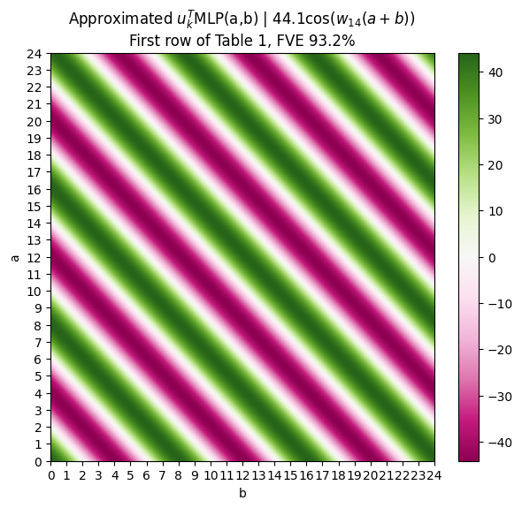
This is just my plot of the function that they wrote down in Table 1. Personally, I think it would have been much more intuitive to plot the actual values $u_k^T\text{MLP}(a,b)$, and show that they have these diagonal patterns, verifying with the 2D DFT later like they do in Table 1.

Then the final ta-da is the fact that this $u_k^T\text{MLP}(a,b)$ thing weights the term $\cos(w_kc)$. Using a nice little trig identity this means that the model is actually calculating $\cos(w_kc)\cos(w_k(a+b))=\cos(w_k(a+b-c))$, which is cute.

But this still doesn’t tell us yet how $a+b$ is computed—only that it exists by the end of the network (which we already knew, due to the fact that the model has good performance), and that $-c$ is sort of built right into the final neuron-logit map $W_L$.

Their neurons partition as well… but how does it work…

Just like we found, they show in Figure 5 that most neurons are well-approximated by a single frequency. The neurons that fire at e.g., frequency $k=14$, write to $\sin(w_k),cos(w_k)$ directions from before(?).

For some reason the code for Figure 5a is missing, but I’m assuming they just fit something to the neuron activations in response to $a$ and in response to $b$ and see that it’s like pretty close? Hm, I’m not sure if they really have a very detailed picture of how this composition happens, whether the trig identities they claimed in Figure 1 are actually being used?